From signal processing to graph algorithms to machine learning, algebraic operations on tensors are a foundational component of many modern compute workloads. In this post, we will try to understand the principal components of what we call a “tensor computation”, or the material implementation of an algebraic equation involving tensors. Let’s take a look at a simple tensor computation:

void gemm(int M, int N, int K,
          const int *A,  // A is M x K
          const int *B,  // B is K x N
          int *Z) {      // Z is M x N
    for (int i = 0; i < M; ++i) {
        for (int j = 0; j < N; ++j) {
            int sum = 0;
            for (int k = 0; k < K; ++k) {
                sum += A[i * K + k] * B[k * N + j];
            }
            Z[i * N + j] = sum;
        }
    }
}

This C code computes the algebraic equation \(Z = A \cdot B\), where \(A\), \(B\), and \(Z\) are matrices (2D tensors). Pretty simple, right?

But wait! Algebra itself doesn’t care that we’re operating on C-style arrays in memory, or that we’re iterating on i before j, or even that we’re iteratively accumulating a single intermediate sum! This specific tensor algorithm (matrix-multiply) could be implemented in many different ways, even staying within C: flip the order of i and j, tile the loop nests for better cache locality, spawn parallel work threads, etc.

The fact that we’ve implemented our GEMM in C has forced us to specify the algorithm imperatively, spelling out an implementation that (we hope) emulates an implicitly specified algorithm. This is in contrast to a declarative specification, where the pure mathematical algorithm is first specified in isolation and orthogonal implementation decisions are made explicitly afterwards.

Let’s take a step back- what are we trying to understand? The mathematical operations? The data representation? How compute is allocated in space and time? Weaving every facet of both algorithm and implementation into one representation (here, C code) makes principled analysis difficult. We can begin to separate our concerns by being explicit about the algorithm without imposing restrictions on how it’s implemented. After specifying the algorithm, as well as how we’re representing the data it operates on, we’ll conclude with a declarative specification (a ‘schedule’) for the material execution of operators within it.

To be clear about terms up-front: I’ll use “algorithm” to describe a purely mathematical/algebraic composition of operations, “operation” to describe a computational primitive (+, *), and “computation” to describe an algorithm coupled with a material (hardware, software) implementation of said algorithm.

A Tidy Algorithmic Representation: Extended Einsums

We can, of course, say that we are computing $$Z = A \cdot B$$ where \(A\), \(B\), and \(Z\) are matrices.

In the analysis of how we implement these algorithms, however, it will pay to be a little more explicit about what primitive operations we’re performing: a scalar operation between elements (multiplication) combined with a reduction (summation) along some axis.

This process is neatly expressed using a notation first used in Einstein’s “The Foundation of the General Theory of Relativity”¹, henceforth referred to as Einsums. Einsums define an algorithm in terms of its point wise output, where a point is given by a coordinate in each ‘rank’ (or axis) of a tensor.

The GEMM we’ve been discussing is defined as such:

$$ Z_{m,n} = \Sigma_k [A_{m,k} \times B_{k,n}] $$

Note the lack of a \(k\) index in the output tensor \(Z\): A reduction is performed over indices not present in the output tensor. Here, the reduction is (implicitly, by convention) a sum. We can, however, choose from a broad spectrum of reduction functions (max, product, etc.) to represent a similarly broad spectrum of tensor algorithms. See section 5.3.2 of The EDGE Language² paper for more details on reductions and how they enable Einsums to be a highly expressive representation.

The explicit reduction (here, \(\Sigma\)) is commonly dropped. $$ Z_{m,n} = A_{m,k} \times B_{k,n} $$

For the sake of brevity, we’ll play a little fast and loose and use the term “Einsum” to refer to these “extended” Einsums for the rest of the post, and have the bounds of reduction implicitly defined based on the shapes of the tensors.

By cascading these Einsums using intermediate tensors, we can represent complex algorithms as well as separate out the scalar operations and reductions within simple ones. For example, below is matrix multiplication represented as a cascade of Einsums, with the scalar multiplication and reductions specified separately.

\[ T_{m,n,k} = A_{m,k} \times B_{k,n} \]

\[ Z_{m,n} = T_{m,n,k} \]

This is mathematically identical to the above example, but makes explicit a multi-phase algorithm (multiplication phase -> reduction phase) which makes the mapping to a multi-phase computation more clear.

Einsums are able to express many core kernels in modern workloads, giving us direct visibility into the operations and their data dependencies. There are more general algorithmic specification languages, such as Halide’s³, but using Einsums gives us a more reasonably scoped and tidy space to analyze. This minimal yet expressive algorithmic representation simplifies analysis by specifying solely the mathematical behavior and true (data) dependencies.

Representing an Algorithm’s Implementation

Now that we know exactly what we’re computing in terms of operations and data dependencies, let’s break down the concerns we saw when implementing our GEMM in C. When performing tensor computations (in both hardware and software), we are concerned with:

1. How involved tensors are orchestrated (flattened, sorted, partitioned) as they ‘flow’ between different parts of the algorithm’s data dependency graph. Our C GEMM did not explicitly manipulate the tensors beyond getting and setting elements, but some orchestration may be done under the hood. For example, unrolling the innermost loop by 4 core effectively partitions the k index into blocks of 4 elements, exposing data-level parallelism which a superscalar processor could take advantage of.

2. How the ranks of tensors are represented in memory (compression, implicit vs. explicit coordinates, etc.). Our C GEMM operates on tensors that are dense (contiguous, uncompressed) and stored in row-major order.

3. Scheduling decisions, such as caching rather than recomputing results, block sizes, and loop order. Our C GEMM computes the entire output matrix row-by-row, accumulating dot product results in a single intermediate variable.

Let’s discuss some structured, declarative representations for these concerns. Combined with the algorithm we’ve declared in the previous section, we’ll have synthesized a tensor computation whose principal characteristics we’ve successfully orthogonalized.

Orchestrating a Tensor Without Saying too Much: Fibertrees

A fibertree represents a tensor as a list of ranks, where a rank is a vector representing one dimension of the tensor. Indexing into a rank vector yields either a set of pointers to nodes in the next lower rank, or a value if that rank is the lowest rank. Note that the ordering of these ranks is a design choice, since it affects the traversal path for accessing points in that tensor. Here’s a graphical example of a fibertree representing a (sparse) tensor with ranks \(M\) and \(K\):

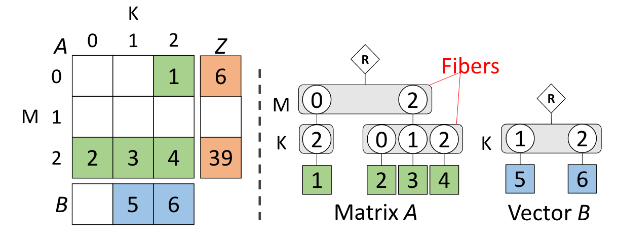
A fiber is defined as “the collection of coordinates that are children of a single coordinate”⁴, or, more simply, the children of a given node in a fibertree.

A fibertree describes a tensor insofar as it tells you how you’d traverse its ranks: A[2][1] in the above matrix, for example, would be located by expanding the 2 fiber in the M rank, and selecting the 1 leaf (with value 3) in the K rank of that fiber. A nice property of fibertrees is that they naturally capture sparsity, a critical consideration on practical datasets (social graphs as an extreme example), by simply ending fibers when all downstream points are null. The implementation of searching through a rank and chasing pointers down fibers are left to the in-memory rank representation, discussed in the next section.

Manipulating these fibertrees (fusing, splitting, or changing the order of ranks) encompass content-preserving transformations on tensors. A content-preserving transformation does not change the leaf/‘true’ values of a tree/tensor. Observe that these content-preserving transformations model data orchestration in an accelerator. Content-preserving here means that the original coordinate to value mapping (the content) of the tensor is preserved. Partitioning a tensor is represented as so:

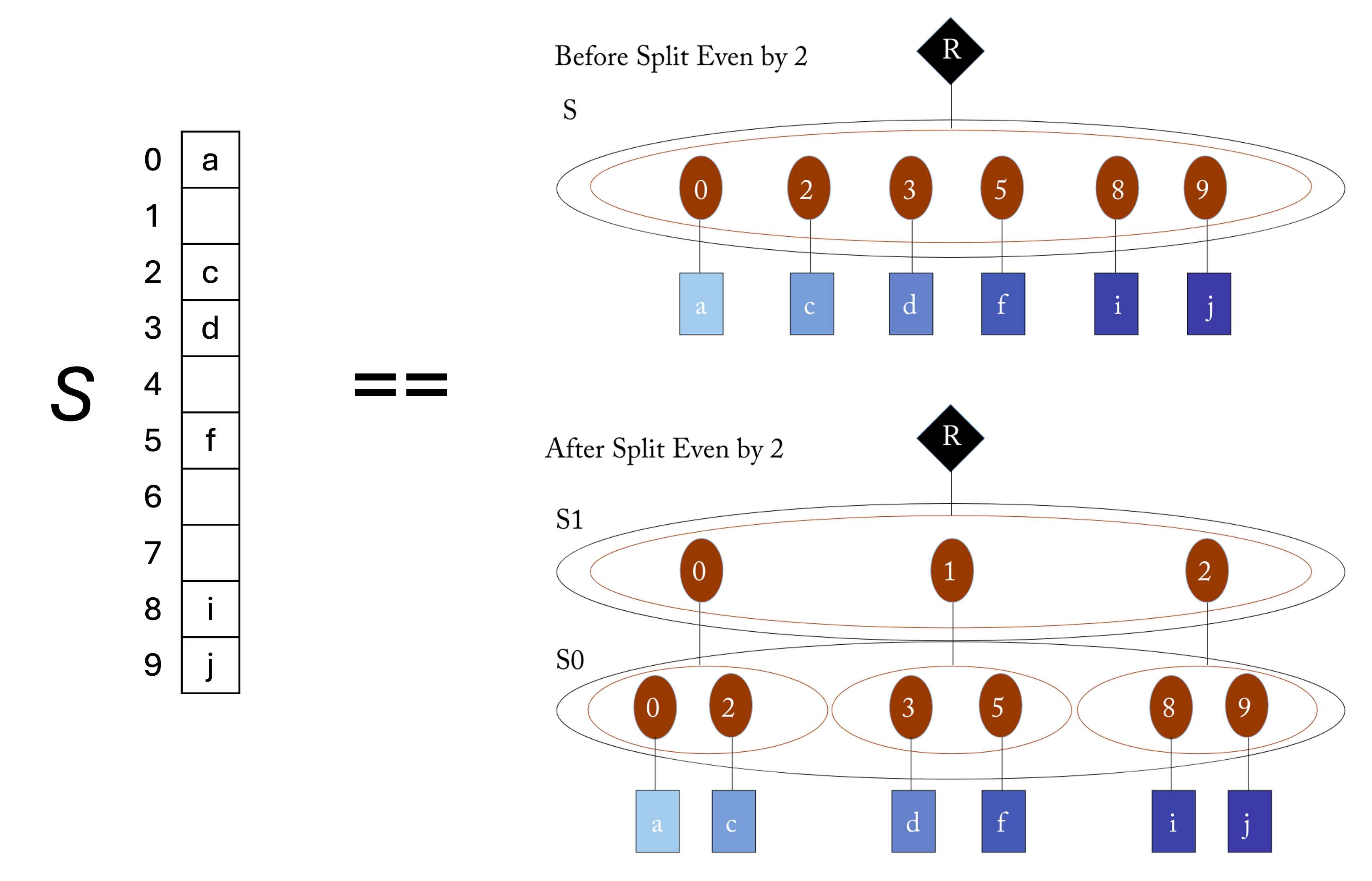
The two fibertrees represent the same (sparse) vector \(S\), but the split (partitioned) fibertree creates a new, coarser dimension over which parallel threads can operate while maintaining spatial locality. These transformations allow us to express many dataflow orchestration decisions without introducing undue implementation constraints on the algorithm nor the underlying representation of each rank of the tensor.

Of course, any practical realization of this concept must enforce an interface through which these manipulations are specified, but the fibertree abstraction itself imposes no such restriction.

Tensors in Memory

In addition to dense representations (contiguous, blocked, etc.), there are many compressed formats for the ranks of a tensor that exploit sparsity to reduce pressure on memory bandwidth (eliding transmitting zeroes) and arithmetic units (eliding explicitly multiplying, adding, etc. with zeroes). CSR (compressed sparse row), a popular compressed tensor format, is illustrated below for a sparse rank-2 tensor, along with traditional matrix notation and as an abstract fibertree.

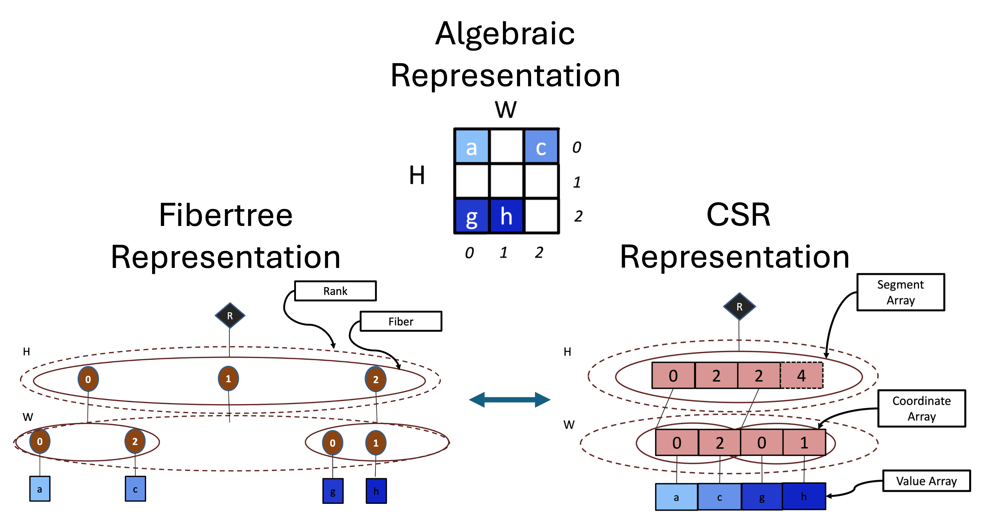
This in-memory representation materializes the ranks of a fibertree, culminating in a material, flexible, and expressive specification for the representation of data (and how it is accessed) in tensor computations.

Scheduling Decisions

“Scheduling” a loop nest encompasses a broad range of decisions related to when and where operations occur throughout the execution of an algorithm. We can broadly classify scheduling decisions into

• The granularity of interleaving operations between stages (scheduling in time)
• Loop ordering
• Loop vectorization/blocking (scheduling in space)

Here’s an example schedule in the Halide³ scheduling language:

// 1D normalized blur algorithm
bh(x) = in(x-1) + in(x) + in(x+1);
bd(x) = bh(x)/3;

// Schedule
bd.tile(x, xi, 32) .vectorize(xi, 8);
bh.compute_at(bd, xi).vectorize(x, 8);

This code schedules two stages bh and bd, and can be interpreted as

For each tile of 32 `bd` elements {
    compute 32 elements of `bh`, 8 at a time
    compute the 32 `bd` elements from those `bh` elements, 8 at a time
}

Here the hardware that this schedule executes on is not described, since Halide was designed to compile kernels for a given architecture. Hardware resources (how wide the datapath is, which and how many processing elements are available, etc.) would be explicitly described as a part of the schedule if the hardware itself was a part of the design space.

Note that in practice, high-level declarative scheduled compilers such as Halide requires a lot of seemingly-boring but critical bounds inference and edge case handling, such as making sure dependencies are computed when their indices lie over a tile boundary. For example, if in were explicitly loaded into memory tile-by-tile, we’d have to handle the case when in(x+1) lies over a tile boundary.

Putting it all together

We have now defined declarative representations for

• The mathematical algorithm (via Einsums)
• How a tensor’s ranks are traversed (via fibertrees)
• How those ranks are represented in memory
• When and where operations occur (via a schedule)

Which can be combined to synthesize the material computation being performed.

While this declarative framework cannot necessarily express more of the design space than an imperative one, the separation of concerns lends itself to both expressive and principled modeling of accelerators ⁵, as well as more agile design (for example, of image processing kernels across heterogeneous hardware platforms³ ).